

會從最多學習資源, 且簡單易學, 又支援多種程式語言, 所以選擇 Google TensorFlow,
而 Keras 又是基於 TensorFlow, 提供更高階 API, 相對於 TensorFlow 更易學習,
且 Keras 本身也內建提供了 AI 訓練資料集 (英文官網、中文官網),
節省了 AI 初學者準備大量資料的時間,
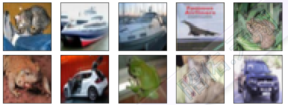
而這次是利用 Cifar10 物體圖片集,
也就是要讓 AI 辨識圖片是什麼物體, 範例如下 :
至於「AI 與機器學習」的觀念, 可以參考 Google 釋出的內部培訓教材 :
點選此處: 《Google 內部培訓教材》Machine Learning Crash Course 機器學習速成課程(影片可選擇顯示中文字幕).
點選此處: 《Google 內部培訓教材》Learn with Google AI(影片可選擇顯示字幕;若無中文字幕,也可選擇自動翻譯字幕).
點選此處: TensorFlow 支援 Python 最完整, 且 Python 易學、應用廣泛, 建議學習.
那就開始用「CNN 卷積神經網路」來辨識「Cifar10 物體圖片集」, 其參考步驟, 如下 :
點選此處: 參考我這篇文章【安裝 Google TensorFlow 與 Keras 環境】.
1)透過 Keras 下載 Cifar10 資料集
from keras.datasets import cifar10 #################### # 第一次執行 load_data() 會從網路下載 Cifar10 資料集 # load_data() 會分析 Cifar10 資料集, 且回傳 "二維 Tuple 元組" #################### ((train_feature, train_label), (test_feature, test_label)) = cifar10.load_data()#################### # 查看 train 與 test 的資料描述 #################### print( 'train feature datas =', train_feature.shape ) # 輸出結果: train feature datas = (50000, 32, 32, 3) # 四維陣列, 第一維陣列長度 50000, 第二維陣列長度 32, 第三維陣列長度 32, 第四維陣列長度 3 # 說明: 訓練用的圖片資料有 50000 筆, 每筆長寬為 32x32 且為 RGB 三原色的彩色圖片 print( 'test feature datas =', test_feature.shape ) # 輸出結果: test feature datas = (10000, 32, 32, 3) # 四維陣列, 第一維陣列長度 10000, 第二維陣列長度 32, 第三維陣列長度 32, 第四維陣列長度 3 # 說明: 測試用的圖片資料有 10000 筆, 每筆長寬為 32x32 且為 RGB 三原色的彩色圖片
2)將 Cifar10 訓練資料的二維圖片,收斂顏色數值
####################
# Cifar10 提供的圖片格式為 32 x 32 x 3 (3 表示 RGB 三原色)
# CNN 輸入層的每筆 Data 都是三維陣列
# 且 Train Feature 所有圖片, 每個本身就是三維陣列, 不用進行轉換
# RGB 顏色數值為 0~255, 除以 255, 讓顏色數值收斂到 0~1, 會讓後續訓練模型時, 可以提高準確率
####################
train_feature_vector = train_feature / 255

# 查看 feature vector 集合
print( 'train feature vector datas =', train_feature_vector.shape )
# 輸出結果:
train feature vector datas = (50000, 32, 32, 3)
3)將 Cifar10 訓練資料的真實數值,轉換為 One-Hot Encoding
####################
# CNN 輸出層的每筆 Data 都是一維陣列
# 所以, 需將 Train Label 資料轉換為 One-Hot Encoding, 也就是
# 1 轉換為 [0, 1, 0, 0, 0, 0, 0, 0, 0, 0]
# 5 轉換為 [0, 0, 0, 0, 0, 1, 0, 0, 0, 0]
# 9 轉換為 [0, 0, 0, 0, 0, 0, 0, 0, 0, 1]
####################
from keras.utils import np_utils

train_label_onehot = np_utils.to_categorical(train_label)
4)建立 Convolutional Neural Network(CNN 卷積神經網路) Model 模型
####################
# 載入所需的相關套件
####################
from keras.models import Sequential
from keras.layers import Conv2D, MaxPooling2D, Flatten, Dense

####################
# 建立 Sequential 順序模組
####################
model = Sequential()

####################
# 模型加入【輸入層】與【第一層卷積層】
####################
model.add( Conv2D( input_shape = (32, 32, 3)     # 輸入層為 (32, 32, 3) 的三維陣列
                 , filters = 8                   # 產生 8 個類似濾鏡效果的卷積圖片
                                                 # (值越大, 卷積圖片越多, 訓練越精準, 相對訓練時間也越久)
                 , kernel_size = (5, 5)          # 卷積圖片採用 5x5 filter weight 進行卷積運算
                 , padding = 'same'              # 卷積圖片大小與原始圖片一樣, 也就是 32x32
                 , activation = 'relu'           # 使用 relu 激活函數
                 )
         )

####################
# 模型加入【第一層池化層】
####################
model.add( MaxPooling2D( pool_size = (2, 2) ) )    # 以 2x2 進行縮減取樣
                                                   # (卷積圖片若為 32x32, 則縮減取樣後的圖片為 16x16)

####################
# 模型加入【平坦層】
# 接下來的 layer 屬於【MLP 多層感知】,所以,需透過【平坦層】將多維度陣列轉換為一維陣列
####################
model.add( Flatten() )

####################
# 模型加入【隱藏層】
# 「隱藏層」可以有多層, 可比喻為「AI 人數」
# 「units 神經元」可比喻為「AI 智力」
####################
model.add( Dense( units = 256                   # 隱藏層有 256 個神經元 (值越大, 訓練越精準, 相對訓練時間也越久)
                , kernel_initializer = 'normal' # 使用 normal 初始化 weight 權重與 bias 偏差值
                , activation = 'relu'           # 使用 relu 激活函數
                )
         )

####################
# 模型加入【輸出層】
####################
model.add( Dense( units = 10                    # 輸出層有 10 個神經元 (因為數字只有 0 ~ 9)
                , kernel_initializer = 'normal' # 使用 normal 初始化 weight 權重與 bias 偏差值
                , activation = 'softmax'        # 使用 softmax 激活函數 (softmax 值越高, 代表機率越大)
                )
         )
5)Model 模型進行【Train 訓練】
#################### # 設定模型的訓練方式 #################### model.compile( loss='categorical_crossentropy' # 設定 Loss 損失函數 為 categorical_crossentropy , optimizer = 'adam' # 設定 Optimizer 最佳化方法 為 adam , metrics = ['accuracy'] # 設定 Model 評估準確率方法 為 accuracy ) #################### # 開始訓練 # CNN 輸入層的每筆 Data 都是三維陣列, 這就是為何 x 輸入 train_feature 或 train_feature_vector 皆可 # CNN 輸出層的每筆 Data 都是一維陣列, 這就是為何 y 輸入 train_label_onehot, 而非 train_label # (若準確率不高, 改善 1: 可再執行這個函數, 進行重覆訓練) # (若準確率不高, 改善 2: 重新建立 Model, 且增加 卷積層 filter 數, 重新進行訓練) # (若準確率不高, 改善 3: 重新建立 Model, 且增加 隱藏層 units 神經元數, 重新進行訓練) # (若準確率不高, 改善 4: 重新建立 Model, 且增加 隱藏層 layer, 重新進行訓練) # (若準確率不高, 改善 5: 重新建立 Model, 且更換訓練方式(神經網路), 重新進行訓練) #################### history = model.fit( # 訓練的歷史記錄, 會會回傳到指定變數 history x = train_feature_vector # 設定 圖片 Features 特徵值 (cifar10 提供 50000 筆資料) , y = train_label_onehot # 設定 圖片 Label 真實值 (cifar10 提供 50000 筆資料) , validation_split = 0.2 # 設定 有多少筆驗證 (50000*0.2=10000 筆驗證, 50000*0.8=40000 筆訓練) , epochs = 30 # 設定 訓練次數 (值 10 以上, 值越大, 訓練時間越久, 但訓練越精準) , batch_size = 1000 # 設定 訓練時每批次有多少筆 (值 100 以上, 值越大, 訓練速度越快, 但需記憶體要夠大) , verbose = 2 # 是否 顯示訓練過程 (0: 不顯示, 1: 詳細顯示, 2: 簡易顯示) ) # 執行的顯示結果 (這會花一些時間, 然後會逐次顯示訓練結果) # loss: 使用訓練資料, 得到的損失函數誤差值 (值越小, 代表準確率越高) # acc: 使用訓練資料, 得到的評估準確率 (值在 0~1, 值越大, 代表準確率越高) # val_loss: 使用驗證資料, 得到的損失函數誤差值 (值越小, 代表準確率越高) # val_acc: 使用驗證資料, 得到的評估準確率 (值在 0~1, 值越大, 代表準確率越高) # 這是 epochs=30, batch_size=1000, verbose=2 顯示【簡易結果】...

6)顯示 Train History 訓練歷史記錄的準確率圖表
#################### # 定義函數, 用來顯示訓練歷史記錄的圖表 #################### import matplotlib.pyplot as plot # plot 可以視為畫布 def train_history_graphic( history # 資料集合 , history_key1 # 資料集合裡面的來源 1 (有 loss, acc, val_loss, val_acc 四種) , history_key2 # 資料集合裡面的來源 2 (有 loss, acc, val_loss, val_acc 四種) , y_label # Y 軸標籤文字 ) : # 資料來源 1 plot.plot( history.history[history_key1] ) # 資料來源 2 plot.plot( history.history[history_key2] ) # 標題 plot.title( 'train history' ) # X 軸標籤文字 plot.xlabel( 'epochs' ) # Y 軸標籤文字 plot.ylabel( y_label ) # 設定圖例 # (參數 1 為圖例說明, 有幾個資料來源, 就對應幾個圖例說明) # (參數 2 為圖例位置, upper 為上面, lower 為下面, left 為左邊, right 為右邊) plot.legend( ['train', 'validate'] , loc = 'upper left' ) # 顯示畫布 plot.show() #################### # 顯示 train history 準確率圖表 #################### train_history_graphic( history, 'acc', 'val_acc', 'accuracy' ) # 輸出結果 (可以得知, 隨著訓練次數的增加, 準確率也越來越高) :#################### # 顯示 train history 損失函數誤差值圖表 #################### train_history_graphic( history, 'loss', 'val_loss', 'loss' ) # 輸出結果 (可以得知, 隨著訓練次數的增加, 誤差值率也越來越低) :

7)用【訓練好的 Model】拿【Cifar10 測試資料】來評估【Model 準確率】
####################
# CNN 輸入層的每筆 Data 都是三維陣列
# 且 Test Feature 所有圖片, 每個本身就是三維陣列, 不用進行轉換
# RGB 顏色數值為 0~255, 除以 255, 讓顏色數值收斂到 0~1, 會讓後續模型預測時, 可以提高準確率
####################
test_feature_vector = test_feature / 255

####################
# CNN 輸出層的每筆 Data 都是一維陣列
# 所以, 需將 Test Label 資料轉換為 One-Hot Encoding
####################
test_label_onehot = np_utils.to_categorical(test_label)

####################
# 使用測試資料評估 Model 的【損失函數誤差值】與【準確率】
####################
eval = model.evaluate( test_feature_vector, test_label_onehot )

# 顯示 Model 評估測試資料的【損失函數誤差值】與【準確率】
print( 'loss =', eval[0] )
print( 'accuracy =', eval[1] )

# 輸出結果 (0.6044 準確率表示 10000 筆資料, 會對 6044 筆, 會錯 3956 筆) :
loss = 1.1440551203727722
accuracy = 0.6044  # 在相同的神經元數量, 比之前用「MLP 多層感知」得到的 0.4905 準確率高出許多
8)用【訓練好的 Model】拿【Cifar10 測試資料】進行【辨識物體圖片】
####################
# 用【訓練好的 Model】進行【辨識物體圖片】
####################
prediction = model.predict_classes( test_feature )

####################
# 顯示圖片集全部的預測結果
# 顯示圖片集第 340 ~ 360 筆的預測結果
####################
print( prediction )
print( prediction[340:360] )

# 輸出結果 :
[3 8 0 ... 5 1 7]
[4 6 2 7 8 5 7 6 8 9 9 1 8 2 2 4 2 2 1 0]

####################
# 將 Prediction 數值轉換成 Prediction 說明文字
####################
# Label 數值對應的說明文字
label_desc = [ 'airplane', 'automobile', 'bird', 'cat', 'deer', 'dog', 'frog', 'horse', 'ship', 'truck' ]

# Prediction 數值轉換成 Prediction 說明文字
prediction_desc = list( map( lambda x : label_desc[x], prediction ) )

# 顯示圖片集第 340 ~ 360 筆的預測結果
print( prediction_desc[340:360] )
# 輸出結果 :
['deer', 'frog', 'bird', 'horse', 'ship', 'bird', 'horse', 'frog', 'ship', 'truck', 'truck', 'automobile', 'ship', 'bird', 'bird', 'deer', 'bird', 'deer', 'automobile', 'ship']
9)預測結束後, 接下來試著找出預測錯誤的資料
#################### # 透過 DataFrame 對照表清單, 來顯示 Label 真實數值, 與 AI 預設結果 #################### import pandas as pd # Pandas.DataFrame 的資料集需要一維陣列, 而 test_label 本身是二維陣列, 需透過 reshape 轉換為一維陣列 test_label_onearr = test_label.reshape(len(test_label)) checkList = pd.DataFrame( {'label':test_label_onearr # Column1 名稱: 欄位值集合 (這裡提供 Label 真實數值) ,'prediction':prediction # Column2 名稱: 欄位值集合 (這裡提供 AI 預測結果) } ) # 顯示對照表前 10 筆結果 print( checkList[0:10] )#################### # 列出對照表中, prediction 欄位值 不等於 label 欄位值的資料 #################### checkList[ checkList.prediction != checkList.label ]
.....
#################### # 定義函數, 用來顯示 Cifar10 多筆影像, 真實數值, 與 AI 預設結果 #################### import matplotlib.pyplot as plot # plot 可以視為畫布 import math def show_feature_label_prediction( features , labels , predictions , indexList # 資料集合中, 要顯示的索引陣列 ) : # 要顯示的索引陣列長度 num = len(indexList) # 設定畫布的寬(參數 1)與高(參數 2) plot.gcf().set_size_inches( 2*5, (2+0.4)*math.ceil(num/5) ) loc = 0 for i in indexList : # 目前要在畫布上的哪個位置顯示 (從 1 開始) loc += 1 # 畫布區分為幾列(參數 1), 幾欄(參數 2), 目前在哪個位置(參數 3) subp = plot.subplot( math.ceil(num/5), 5, loc ) # 畫布上顯示圖案, 其中 cmap=binary 為顯示黑白圖案 subp.imshow( features[i], cmap='binary' ) # 設定標題內容 # 有 AI 預測結果資料, 才在標題顯示預測結果 if( len(predictions) > 0 ) : title = 'ai = ' + label_desc[ predictions[i] ] title += (' (o)' if predictions[i]==labels[i] else ' (x)') # 預測正確顯示(o), 錯誤顯示(x) title += '\nlabel = ' + label_desc[ labels[i] ] # 沒有 AI 預測結果資料, 則只在標題顯示真實數值 else : title = 'label = ' + label_desc[ labels[i] ] # 在畫布上顯示標題, 且字型大小為 12 subp.set_title( title, fontsize=12 ) # X, Y 軸不顯示刻度 subp.set_xticks( [] ) subp.set_yticks( [] ) # 顯示畫布 plot.show() #################### # 從測試資料集第 0 位置, 顯示 10 個資料的圖片, 真實數值, 與預測結果 #################### show_feature_label_prediction( test_feature, test_label_onearr, prediction, range(0, 10) ) # 輸出結果 :
# 可以改版為顯示中文, 且預測錯誤顯示紅色字體 :
#################### # 之前評估 Model 準確率為 0.6044, 也就是 10000 筆資料, 會對 6044 筆, 會錯 3956 筆 # 將這些錯誤資料顯示出來, 看看是否為圖形太混亂不清楚, 從而了解 AI 為何會預測錯誤 # 另外, 可以藉由【提高訓練次數】或【增加卷積層的 filter 數】或【增加隱藏層的神經元數】 # 或【增加隱藏層】或【改變神經網路方式】, 來提升 AI 準確率 #################### # 顯示預測錯誤的前 20 筆資料 show_feature_label_prediction( test_feature , test_label_onearr , prediction , checkList.index[checkList.prediction != checkList.label][0:20] )

10)將訓練好的 Model 模型儲存起來, 在日後可以直接載入使用, 而不用再重新訓練
####################
# 將 Model 模型儲存成 HDF5 檔案, 路徑名稱為 D 槽下的 my_cifar10_cnn_model.h5
# 檔案命名規則: 資料集名稱_神經網路名稱_model.h5
####################
model.save('d:/my_cifar10_cnn_model.h5')

####################
# 從 D 槽下的 my_cifar10_cnn_model.h5 檔案, 載入 Model 模型
####################
from keras.models import load_model

model = load_model('d:/my_cifar10_cnn_model.h5')
以上, 參考看看囉, 如有任何問題, 也歡迎一同一起研究 ^ ^
